
Vitalik Buterin through the Vitalik Buterin Weblog
It is a mirror of the put up at https://medium.com/@VitalikButerin/exploring-elliptic-curve-pairings-c73c1864e627
Set off warning: math.
One of many key cryptographic primitives behind varied constructions, together with deterministic threshold signatures, zk-SNARKs and different less complicated types of zero-knowledge proofs is the elliptic curve pairing. Elliptic curve pairings (or “bilinear maps”) are a current addition to a 30-year-long historical past of utilizing elliptic curves for cryptographic functions together with encryption and digital signatures; pairings introduce a type of “encrypted multiplication”, significantly increasing what elliptic curve-based protocols can do. The aim of this text shall be to enter elliptic curve pairings intimately, and clarify a common define of how they work.
You’re not anticipated to know every little thing right here the primary time you learn it, and even the tenth time; these items is genuinely arduous. However hopefully this text provides you with a minimum of a little bit of an thought as to what’s going on underneath the hood.
Elliptic curves themselves are very a lot a nontrivial subject to know, and this text will typically assume that you know the way they work; if you don’t, I like to recommend this text right here as a primer: https://weblog.cloudflare.com/a-relatively-easy-to-understand-primer-on-elliptic-curve-cryptography/. As a fast abstract, elliptic curve cryptography includes mathematical objects known as “factors” (these are literal two-dimensional factors with (�,�) coordinates), with particular formulation for including and subtracting them (ie. for calculating the coordinates of �=�+�), and you too can multiply some extent by an integer (ie. �⋅�=�+�+…+�, although there’s a a lot quicker strategy to compute it if � is massive).
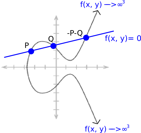
Right here’s how level addition seems to be like graphically.
There exists a particular level known as the “level at infinity” (�), the equal of zero in level arithmetic; it’s at all times the case that �+�=�. Additionally, a curve has an “order“; there exists a quantity � such that �⋅�=� for any � (and naturally, �⋅(�+1)=�,�⋅(7⋅�+5)=�⋅5, and so forth). There’s additionally some generally agreed upon “generator level” �, which is known to in some sense symbolize the #1. Theoretically, any level on a curve (besides �) might be �; all that issues is that � is standardized.
Pairings go a step additional in that they help you verify sure sorts of extra sophisticated equations on elliptic curve factors — for instance, if �=�⋅�,�=�⋅� and �=�⋅�, you’ll be able to verify whether or not or not �⋅�=�, having simply �,� and � as inputs. This may seem to be the basic safety ensures of elliptic curves are being damaged, as details about � is leaking from simply understanding P, but it surely seems that the leakage is extremely contained — particularly, the decisional Diffie Hellman downside is straightforward, however the computational Diffie Hellman downside (understanding � and � within the above instance, computing �=�⋅�⋅�) and the discrete logarithm downside (recovering � from �) stay computationally infeasible (a minimum of, in the event that they had been earlier than).
A 3rd method to have a look at what pairings do, and one that’s maybe most illuminating for many of the use circumstances that we’re about, is that if you happen to view elliptic curve factors as one-way encrypted numbers (that’s, �������(�)=�⋅�=�), then whereas conventional elliptic curve math permits you to verify linear constraints on the numbers (eg. if �=�⋅�,�=�⋅� and �=�⋅�, checking 5⋅�+7⋅�=11⋅� is actually checking that 5⋅�+7⋅�=11⋅�), pairings allow you to verify quadratic constraints (eg. checking �(�,�)⋅�(�,�⋅5)=1 is actually checking that �⋅�+5=0). And going as much as quadratic is sufficient to allow us to work with deterministic threshold signatures, quadratic arithmetic packages and all that different great things.
Now, what is that this humorous �(�,�) operator that we launched above? That is the pairing. Mathematicians additionally generally name it a bilinear map; the phrase “bilinear” right here principally signifies that it satisfies the constraints:
�(�,�+�)=�(�,�)⋅�(�,�)
�(�+�,�)=�(�,�)⋅�(�,�)
Word that + and ⋅ might be arbitrary operators; whenever you’re creating fancy new sorts of mathematical objects, summary algebra doesn’t care how + and ⋅ are outlined, so long as they’re constant within the standard methods, eg. �+�=�+�,(�⋅�)⋅�=�⋅(�⋅�) and (�⋅�)+(�⋅�)=(�+�)⋅�.
If �, �, � and � had been easy numbers, then making a easy pairing is straightforward: we will do �(�,�)=2��. Then, we will see:
�(3,4+5)=23⋅9=227
�(3,4)⋅�(3,5)=23⋅4⋅23⋅5=212⋅215=227
It’s bilinear!
Nevertheless, such easy pairings are usually not appropriate for cryptography as a result of the objects that they work on are easy integers and are too straightforward to research; integers make it straightforward to divide, compute logarithms, and make varied different computations; easy integers haven’t any idea of a “public key” or a “one-way perform”. Moreover, with the pairing described above you’ll be able to go backwards – understanding �, and understanding �(�,�), you’ll be able to merely compute a division and a logarithm to find out �. We would like mathematical objects which might be as shut as attainable to “black bins”, the place you’ll be able to add, subtract, multiply and divide, however do nothing else. That is the place elliptic curves and elliptic curve pairings are available.
It seems that it’s attainable to make a bilinear map over elliptic curve factors — that’s, provide you with a perform �(�,�) the place the inputs � and � are elliptic curve factors, and the place the output is what’s known as an (��)12 ingredient (a minimum of within the particular case we are going to cowl right here; the specifics differ relying on the main points of the curve, extra on this later), however the math behind doing so is kind of advanced.
First, let’s cowl prime fields and extension fields. The beautiful elliptic curve within the image earlier on this put up solely seems to be that method if you happen to assume that the curve equation is outlined utilizing common actual numbers. Nevertheless, if we truly use common actual numbers in cryptography, then you need to use logarithms to “go backwards”, and every little thing breaks; moreover, the quantity of house wanted to really retailer and symbolize the numbers could develop arbitrarily. Therefore, we as a substitute use numbers in a prime discipline.
A first-rate discipline consists of the set of numbers 0,1,2…�−1, the place � is prime, and the assorted operations are outlined as follows:
�+�:(�+�) % �
�⋅�:(�⋅�) % �
�−�:(�−�) % �
�/�:(�⋅��−2) % �
Mainly, all math is completed modulo � (see right here for an introduction to modular math). Division is a particular case; usually, 32 just isn’t an integer, and right here we wish to deal solely with integers, so we as a substitute attempt to discover the quantity � such that �⋅2=3, the place ⋅ after all refers to modular multiplication as outlined above. Due to Fermat’s little theorem, the exponentiation trick proven above does the job, however there may be additionally a quicker strategy to do it, utilizing the Prolonged Euclidean Algorithm. Suppose �=7; listed below are a number of examples:
2+3=5 % 7=5
4+6=10 % 7=3
2−5=−3 % 7=4
6⋅3=18 % 7=4
3/2=(3⋅25) % 7=5
5⋅2=10 % 7=3
In case you mess around with this type of math, you’ll discover that it’s completely constant and satisfies the entire standard guidelines. The final two examples above present how (�/�)⋅�=�; you too can see that (�+�)+�=�+(�+�),(�+�)⋅�=�⋅�+�⋅�, and all the opposite highschool algebraic identities and love proceed to carry true as effectively. In elliptic curves in actuality, the factors and equations are normally computed in prime fields.
Now, let’s discuss extension fields. You have got most likely already seen an extension discipline earlier than; the commonest instance that you simply encounter in math textbooks is the sphere of advanced numbers, the place the sphere of actual numbers is “prolonged” with the extra ingredient −1=�. Mainly, extension fields work by taking an current discipline, then “inventing” a brand new ingredient and defining the connection between that ingredient and current parts (on this case, �2+1=0), ensuring that this equation doesn’t maintain true for any quantity that’s within the unique discipline, and looking out on the set of all linear combos of parts of the unique discipline and the brand new ingredient that you’ve simply created.

We will do extensions of prime fields too; for instance, we will lengthen the prime discipline mod7 that we described above with �, after which we will do:
(2+3�)+(4+2�)=6+5�
(5+2�)+3=1+2�
(6+2�)⋅2=5+4�
4�⋅(2+�)=3+�
That final end result could also be a bit arduous to determine; what occurred there was that we first decompose the product into 4�⋅2+4�⋅�, which provides 8�−4, after which as a result of we’re working in mod7 math that turns into �+3. To divide, we do:
�/�:(�⋅�(�2−2)) % �
Word that the exponent for Fermat’s little theorem is now �2 as a substitute of �, although as soon as once more if we wish to be extra environment friendly we will additionally as a substitute lengthen the Prolonged Euclidean Algorithm to do the job. Word that ��2−1=1 for any � on this discipline, so we name �2−1 the “order of the multiplicative group within the discipline”.
With actual numbers, the Basic Theorem of Algebra ensures that the quadratic extension that we name the advanced numbers is “full” — you can’t lengthen it additional, as a result of for any mathematical relationship (a minimum of, any mathematical relationship outlined by an algebraic method) you could provide you with between some new ingredient � and the prevailing advanced numbers, it’s attainable to provide you with a minimum of one advanced quantity that already satisfies that relationship. With prime fields, nevertheless, we wouldn’t have this concern, and so we will go additional and make cubic extensions (the place the mathematical relationship between some new ingredient � and current discipline parts is a cubic equation, so 1,� and �2 are all linearly impartial of one another), higher-order extensions, extensions of extensions, and so forth. And it’s these sorts of supercharged modular advanced numbers that elliptic curve pairings are constructed on.
For these all in favour of seeing the precise math concerned in making all of those operations written out in code, prime fields and discipline extensions are applied right here: https://github.com/ethereum/py_pairing/blob/grasp/py_ecc/bn128/bn128_field_elements.py
Now, on to elliptic curve pairings. An elliptic curve pairing (or slightly, the particular type of pairing we’ll discover right here; there are additionally different kinds of pairings, although their logic is pretty comparable) is a map �2×�1→��, the place:
- �1 is an elliptic curve, the place factors fulfill an equation of the shape �2=�3+�, and the place each coordinates are parts of �� (ie. they’re easy numbers, besides arithmetic is all executed modulo some prime quantity)
- �2 is an elliptic curve, the place factors fulfill the identical equation as �1, besides the place the coordinates are parts of (��)12 (ie. they’re the supercharged advanced numbers we talked about above; we outline a brand new “magic quantity” �, which is outlined by a twelfth diploma polynomial like �12−18⋅�6+82=0)
- �� is the kind of object that the results of the elliptic curve goes into. Within the curves that we have a look at, �� is (��)12 (the identical supercharged advanced quantity as utilized in �2)
The primary property that it should fulfill is bilinearity, which on this context signifies that:
- �(�,�+�)=�(�,�)⋅�(�,�)
- �(�+�,�)=�(�,�)⋅�(�,�)
There are two different necessary standards:
- Environment friendly computability (eg. we will make a straightforward pairing by merely taking the discrete logarithms of all factors and multiplying them collectively, however that is as computationally arduous as breaking elliptic curve cryptography within the first place, so it doesn’t depend)
- Non-degeneracy (positive, you could possibly simply outline �(�,�)=1, however that’s not a very helpful pairing)
So how can we do that?
The mathematics behind why pairing features work is kind of difficult and includes fairly a little bit of superior algebra going even past what we’ve seen up to now, however I’ll present a top level view. To start with, we have to outline the idea of a divisor, principally an alternate method of representing features on elliptic curve factors. A divisor of a perform principally counts the zeroes and the infinities of the perform. To see what this implies, let’s undergo a number of examples. Allow us to repair some level �=(��,��), and take into account the next perform:
�(�,�)=�−��
The divisor is [�]+[−�]−2⋅[�] (the sq. brackets are used to symbolize the truth that we’re referring to the presence of the purpose � within the set of zeroes and infinities of the perform, not the purpose P itself; [�]+[�] is not the identical factor as [�+�]). The reasoning is as follows:
- The perform is the same as zero at �, since � is ��, so �−��=0
- The perform is the same as zero at −�, since −� and � share the identical � coordinate
- The perform goes to infinity as � goes to infinity, so we are saying the perform is the same as infinity at �. There’s a technical cause why this infinity must be counted twice, so � will get added with a “multiplicity” of −2 (detrimental as a result of it’s an infinity and never a zero, two due to this double counting).
The technical cause is roughly this: as a result of the equation of the curve is �3=�2+�,� goes to infinity “1.5 instances quicker” than � does to ensure that �2 to maintain up with �3; therefore, if a linear perform contains solely � then it’s represented as an infinity of multiplicity 2, but when it contains � then it’s represented as an infinity of multiplicity 3.
Now, take into account a “line perform”:
��+��+�=0
The place �, � and � are rigorously chosen in order that the road passes by factors � and �. Due to how elliptic curve addition works (see the diagram on the prime), this additionally signifies that it passes by −�−�. And it goes as much as infinity depending on each � and �, so the divisor turns into [�]+[�]+[−�−�]−3⋅[�].
We all know that each “rational perform” (ie. a perform outlined solely utilizing a finite variety of +,−,⋅ and / operations on the coordinates of the purpose) uniquely corresponds to some divisor, as much as multiplication by a relentless (ie. if two features � and � have the identical divisor, then �=�⋅� for some fixed �).
For any two features � and �, the divisor of �⋅� is the same as the divisor of � plus the divisor of � (in math textbooks, you’ll see (�⋅�)=(�)+(�)), so for instance if �(�,�)=��−�, then (�3)=3⋅[�]+3⋅[−�]−6⋅[�]; � and −� are “triple-counted” to account for the truth that �3 approaches 0 at these factors “3 times as rapidly” in a sure mathematical sense.
Word that there’s a theorem that states that if you happen to “take away the sq. brackets” from a divisor of a perform, the factors should add as much as �([�]+[�]+[−�−�]−3⋅[�] clearly suits, as �+�−�−�−3⋅�=�), and any divisor that has this property is the divisor of a perform.
Now, we’re prepared to have a look at Tate pairings. Contemplate the next features, outlined through their divisors:
- (��)=�⋅[�]−�⋅[�], the place � is the order of �1, ie. �⋅�=� for any �
- (��)=�⋅[�]−�⋅[�]
- (�)=[�+�]−[�]−[�]+[�]
Now, let’s have a look at the product ��⋅��⋅��. The divisor is:
�⋅[�]−�⋅[�]+�⋅[�]−�⋅[�]+�⋅[�+�]−�⋅[�]−�⋅[�]+�⋅[�]
Which simplifies neatly to:
�⋅[�+�]−�⋅[�]
Discover that this divisor is of precisely the identical format because the divisor for �� and �� above. Therefore, ��⋅��⋅��=��+�.
Now, we introduce a process known as the “closing exponentiation” step, the place we take the results of our features above (��,��, and so forth.) and lift it to the facility �=(�12−1)/�, the place �12−1 is the order of the multiplicative group in (��)12 (ie. for any �∈(��)12,�(�12−1)=1). Discover that if you happen to apply this exponentiation to any end result that has already been raised to the facility of �, you get an exponentiation to the facility of �12−1, so the end result turns into 1. Therefore, after closing exponentiation, �� cancels out and we get ���⋅���=(��+�)�. There’s some bilinearity for you.
Now, if you wish to make a perform that’s bilinear in each arguments, you want to go into spookier math, the place as a substitute of taking �� of a price straight, you are taking �� of a divisor, and that’s the place the total “Tate pairing” comes from. To show some extra outcomes it’s important to take care of notions like “linear equivalence” and “Weil reciprocity”, and the rabbit gap goes on from there. You will discover extra studying materials on all of this right here and right here.
For an implementation of a modified model of the Tate pairing, known as the optimum Ate paring, see right here. The code implements Miller’s algorithm, which is required to really compute ��.
Word that the actual fact pairings like this are attainable is considerably of a blended blessing: on the one hand, it signifies that all of the protocols we will do with pairings turn out to be attainable, however can be signifies that we’ve to be extra cautious about what elliptic curves we use.
Each elliptic curve has a price known as an embedding diploma; primarily, the smallest � such that ��−1 is a a number of of � (the place � is the prime used for the sphere and � is the curve order). Within the fields above, �=12, and within the fields used for conventional ECC (ie. the place we don’t care about pairings), the embedding diploma is commonly extraordinarily giant, to the purpose that pairings are computationally infeasible to compute; nevertheless, if we’re not cautious then we will generate fields the place �=4 and even 1.
If �=1, then the “discrete logarithm” downside for elliptic curves (primarily, recovering � understanding solely the purpose �=�⋅�, the issue that it’s important to resolve to “crack” an elliptic curve non-public key) might be lowered into the same math downside over ��, the place the issue turns into a lot simpler (that is known as the MOV assault); utilizing curves with an embedding diploma of 12 or larger ensures that this discount is both unavailable, or that fixing the discrete log downside over pairing outcomes is a minimum of as arduous as recovering a non-public key from a public key “the traditional method” (ie. computationally infeasible). Don’t worry; all commonplace curve parameters have been completely checked for this concern.
Keep tuned for a mathematical clarification of how zk-SNARKs work, coming quickly.
Particular because of Christian Reitwiessner, Ariel Gabizon (from Zcash) and Alfred Menezes for reviewing and making corrections.
- website positioning Powered Content material & PR Distribution. Get Amplified Right now.
- PlatoData.Community Vertical Generative Ai. Empower Your self. Entry Right here.
- PlatoAiStream. Web3 Intelligence. Information Amplified. Entry Right here.
- PlatoESG. Carbon, CleanTech, Power, Atmosphere, Photo voltaic, Waste Administration. Entry Right here.
- PlatoHealth. Biotech and Medical Trials Intelligence. Entry Right here.
- BlockOffsets. Modernizing Environmental Offset Possession. Entry Right here.
- Supply: Plato Knowledge Intelligence.
